Manage Docker Containers on Your Raspberry Pi With Portainer
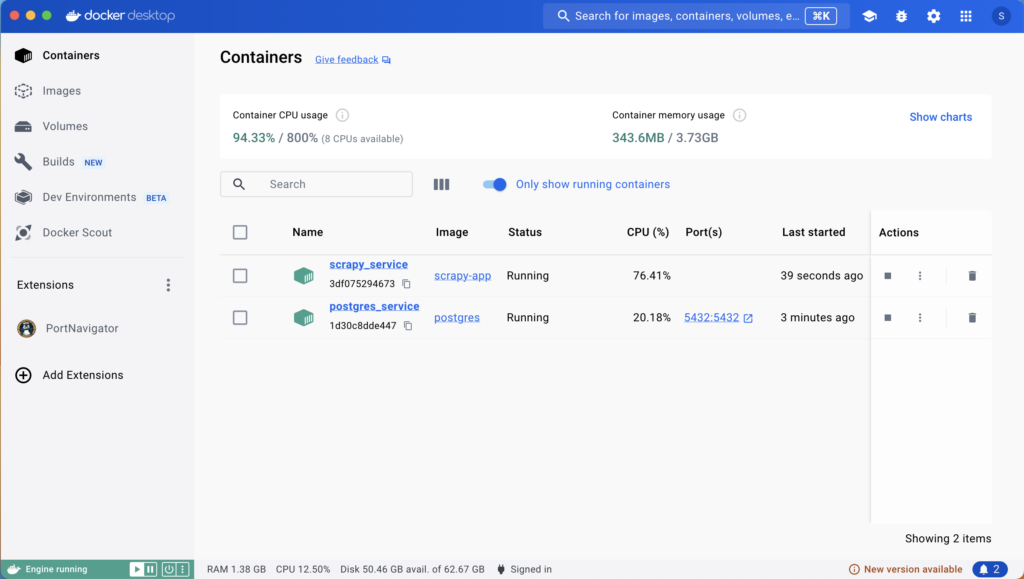
Docker is addictive. As it becomes an indispensable tool in our toolkit, we need a way to streamline container management. Docker offers Docker Desktop, a GUI application, for Mac and Windows users. For Raspberry Pi, I recommend Portainer.
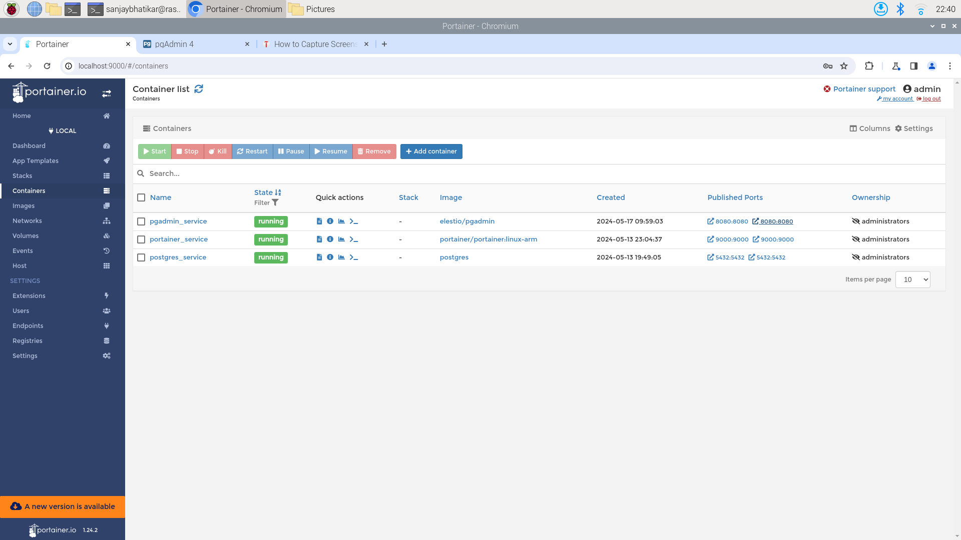
Portainer provides an intuitive web-based interface to manage Docker containers, making it easy to start, stop, modify, or remove containers and monitor usage statistics. It runs in its own container and is well-suited for single-board computers (SBCs) like the Raspberry Pi running Raspbian.
Here’s how to get Portainer up and running on your Raspberry Pi:
- Pull the image:
docker pull portainer/linux-arm - Spin up the container with
docker runcommand like so:
	docker run --name portainer_service --network docker-net \
	-d -p 9000:9000 \
	-v /var/run/docker.sock:/var/run/docker.sock \
	-v ~/Your/path/to/data:/data \
	portainer/portainer:linux-arm
- Access Portainer: Open your web browser and go to http://localhost:9000. That’s it!
Now access Portainer from: http://localhost:9000. That is it!
Deploying AI Models in Real-World Situations
Being an AI practitioner means not only building models but also being familiar with various environments in which these models are deployed. Field applications often leverage platforms such as SBCs. The Raspberry Pi is a popular SBC that runs Linux and integrates seamlessly with various sensors and actuators.
In our FastAI course, you’ll learn from Ph.D. instructors who have invaluable expertise in both model building and the engineering required to deploy these models in real-world situations. We cover essential tools like Docker and Portainer, equipping you with the skills needed to put your AI applications into the hands of users effectively.
Join us to bridge the gap between developing AI models and deploying them in practical environments.


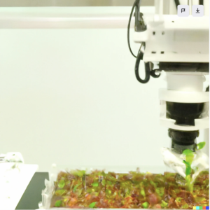 Leveraging pre-trained models and neural transfer learning, we curated an extensive in-house dataset comprising 15,000 images meticulously labeled by cell biologists. These images, capturing various stages of embryonic development, were acquired using both an ordinary DSLR camera and a proprietary hyperspectral imaging robot. Our experimentation precisely determined the optimal timeframe for image acquisition post the initiation of plant transformation, establishing that images from a conventional DSLR were on par with those from the hyperspectral camera for the classification task. The impact of our work extends far beyond the confines of the laboratory, catalyzing a wave of innovations in computer vision within biotechnology R&D, spanning laboratories, greenhouses, and field applications. This progressive integration has not only optimized the R&D pipeline but has also significantly accelerated time-to-market, positioning our consultancy at the forefront of transformative advancements in the biotech sector