Unlocking the Power of Language: Leveraging Large Language Models for Next-Gen Semantic Search and Real-World Applications
Invited talk at Calfus, Pune, June 20, 2024.
I acquired an EC2 instance on Amazon’s cloud for building Generative AI models, gaining access to a Tesla T4 GPU and ample GPU RAM for deploying a Large Language Model (LLM) for an app developed for an investment banking firm. Access to the EC2 instance is primarily through the terminal on my MacBook, which starkly contrasts with the familiar Visual Studio Code (VS Code) environment that offers convenient integrations with GitHub and Docker.
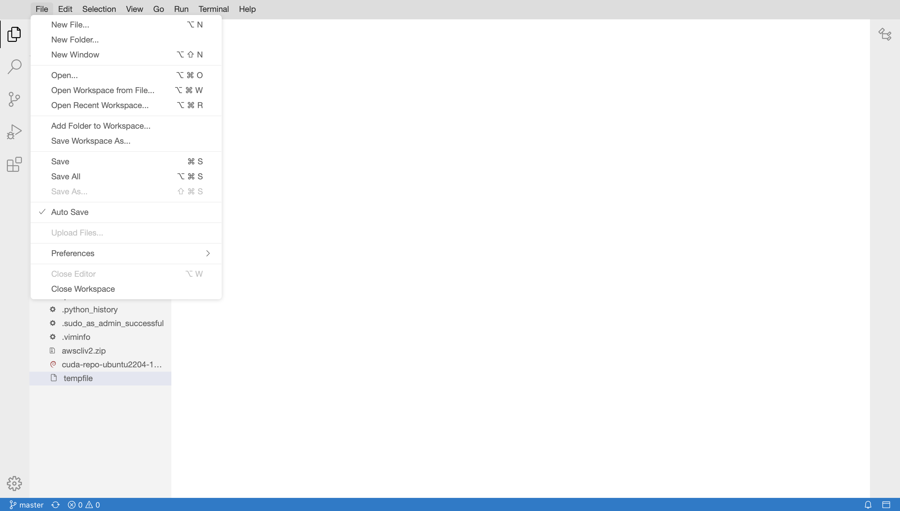
While the Command Line Interface (CLI) is a valuable tool for developers, it can be cumbersome for tasks that benefit from a more visual interface. For quick changes to code moved from development to production environments, the EC2 instance running Ubuntu 22.04 OS offered only the Nano editor. Though Nano is a perfectly good editor, I wanted something closer to VS Code. The solution? A light version of the Theia IDE in Docker, which perfectly met my needs.
To access the EC2 instance, I SSH into it from an open terminal on my MacBook, using a downloaded .pem file for authentication. The command is as follows
ssh -i ~/.ssh/secret.pem deusexmachina@45.245.72.29
A dockerized app typically listens for incoming requests at the host IP address on a specific port. When the app has a web UI, it can be accessed in a web browser using the IP address and port number, allowing access from any location on the web that can reach the IP address.
For our EC2 instance, we can find the required public IP address using AWS CLI. As for the port used by the app, we must ensure it is exposed to the public internet. We will use AWS CLI to check which ports are exposed to the public internet. If the required port is not exposed, we will use AWS CLI to expose it. Ensure you have AWS CLI installed on your computer; if not, follow the instructions here.
aws ec2 describe-security-groups --group-ids sg-08x6bdf6x665XcxeX | \
jq '.SecurityGroups[0].IpPermissions[] | select(.IpRanges[].CidrIp == "0.0.0.0/0")'
The command retrieves information about a specific security group in AWS EC2 and uses jq
to filter the results. Let’s break down each part of the command:
AWS CLI Command
aws ec2 describe-security-groups --group-ids sg-08x6bdf6x665XcxeX
aws ec2 describe-security-groups
: This is an AWS CLI command used to retrieve details about one or more security groups.--group-ids sg-08x6bdf6x665XcxeX
: This option specifies the security group ID for which details are being requested. In this case, the security group ID is sg-08x6bdf6x665XcxeX
.This command outputs information about the specified security group in JSON format.
Piping to jq
| jq '.SecurityGroups[0].IpPermissions[] | select(.IpRanges[].CidrIp == "0.0.0.0/0")'
| jq
: This pipe sends the output of the aws ec2 describe-security-groups
command to jq
, which is a command-line JSON processor..SecurityGroups[0]
: This selects the first (and likely only) security group from the list of security groups returned by the AWS CLI command..IpPermissions[]
: This iterates over each IP permission rule within the selected security group. Each security group can have multiple IP permission rules, which specify which IP ranges are allowed or denied access.select(.IpRanges[].CidrIp == "0.0.0.0/0")
: This select
function filters the IP permission rules to find those that have an IP range (CIDR block) of 0.0.0.0/0
. The 0.0.0.0/0
CIDR block represents the entire IPv4 address space, indicating a rule that applies to all IP addresses.Combining these parts, the full command performs the following actions:
sg-08x6bdf6x665XcxeX
using the AWS CLI.jq
: It processes this JSON output to:0.0.0.0/0
).Here is the JSON indicative of a rule allowing TCP traffic on port 22 (typically used for SSH) from any IP address.
{
"IpProtocol": "tcp",
"FromPort": 22,
"ToPort": 22,
"IpRanges": [
{
"CidrIp": "0.0.0.0/0"
}
],
}
What if the port we need is not open? Here is the command to open a port.
aws ec2 authorize-security-group-ingress --group-id sg-08x6bdf6x665XcxeX \
--protocol tcp --port 8081 --cidr 0.0.0.0/0
The aws ec2 authorize-security-group-ingress
command adds an ingress rule to a specified security group. An ingress rule specifies the type of incoming traffic that is allowed to reach instances associated with the security group. We have used the command with options and arguments as follows:
--group-id sg-08x6bdf6x665XcxeX
: This option specifies the ID of the security group to which you want to add the ingress rule. In this case, the security group ID is sg-08x6bdf6x665XcxeX
.--protocol tcp
: This option specifies the protocol for the rule. Here, tcp
indicates that the rule applies to the TCP protocol.--port 8081
: This option specifies the port number to which the rule applies. In this case, it is port 8081
.--cidr 0.0.0.0/0
: This option specifies the CIDR block (range of IP addresses) that is allowed by this rule. 0.0.0.0/0
represents all IP addresses, meaning the rule allows incoming traffic from any IP address.Putting it all together, the command:
sg-08x6bdf6x665XcxeX
.8081
.0.0.0.0/0
).By running this command, we modify the specified security group to allow incoming TCP traffic on port 8081 from any IP address. In this way, we allow access to an application that is listening on port 8081 to users from anywhere on the internet.
Note on Security:
Allowing traffic from 0.0.0.0/0
means that the port is open to the entire internet. This can be a significant security risk. It is generally advisable to restrict the CIDR range to specific IP addresses or ranges that require access, rather than opening it up to all addresses.
Theia Use Case:
The Theia IDE runs as a web application that listens on port 3000. By running the command: aws ec2 describe-security-groups --group-ids sg-08x6bdf6x665XcxeX | jq '.SecurityGroups[0].IpPermissions[] | select(.IpRanges[].CidrIp == "0.0.0.0/0").FromPort'
, I found that port 3000 was among those open to TCP traffic. However, it was already in use by the web application Grafana. To resolve this, I decided to map port 3000 on Theia’s Docker container to port 3030 on the EC2 instance. I then ran the command to modify the security group, allowing HTTP (or any TCP) traffic to reach Theia on port 3030 from any IP address.
Let’s look at the installation process next.
Here are the steps to install Theia:
docker pull t1m0thyj/theia-alpine
docker run -d --init \
--name theia_service \
--restart always \
-p 3030:3000 \
-v /home/ubuntu:/home/project t1m0thyj/theia-alpine
The docker run
command creates a container named theia_service
and maps port 3030 on the EC2 instance to port 3000 on the container. The image t1m0thyj/theia-alpine
is a lightweight version of the Theia IDE. With the container up and running, as verified by docker ps
, we can access Theia using the URL http://45.245.72.29:3030
in a web browser. Here is what that looks like in Safari on my MacBook.
Using Docker to install Theia IDE on an AWS EC2 instance involves ensuring the container has the necessary permissions to create or update text files on the shared volume. The directory permissions must be correctly set, and it may be necessary to create a user on the container with the same UID/GID as the user on the host. This can be conveniently done with options and arguments passed to the docker run command.
Although the dockerized Theia running on EC2 was accessible this way, it did not allow creating or modifying files. In other words, it functioned as a read-only IDE!
Using Docker to install Theia IDE on an AWS EC2 instance involves ensuring the container has the necessary permissions to create or update text files on the shared volume. The directory permissions must be correctly set, and it may be necessary to create a user on the container with the same UID/GID as the user on the host. Looking into the docker logs with the command docker logs theia_service
on the EC2 machine, it became apparent that the container did not have sufficient permissions on the shared volume.
Ensure that the shared folder between the EC2 host and docker container has the correct ownership and permissions with the following commands:
sudo chown -R ubuntu:ubuntu /home/ubuntu
sudo chmod -R 775 /home/ubuntu
Here, the logged-in user on the EC2 instance has name ubuntu
. This can be verified by running the whoami
command at the terminal prompt. Alternatively, use the $USER
variable in the command like so: sudo chown -R $USER:$USER /home/ubuntu
.
This alone wasn’t enough to fix the issue. Running the whoami
command inside the Docker container from an interactive shell revealed the container user to be theia
. The fix to the permissions error was to ensure that the container user theia
has the same permissions as the instance user ubuntu
. This is possible with a small modification to the options and arguments passed to the docker run
command as follows:
docker run --rm --init \
--name theia_service_temp \
-d -p 3030:3000 \
-v /home/ubuntu/:/home/project \
-u $(id -u ubuntu):$(id -g ubuntu) \
t1m0thyj/theia-alpine
This command spins up a temporary container with --rm
for testing the approach. The container is removed upon exit.
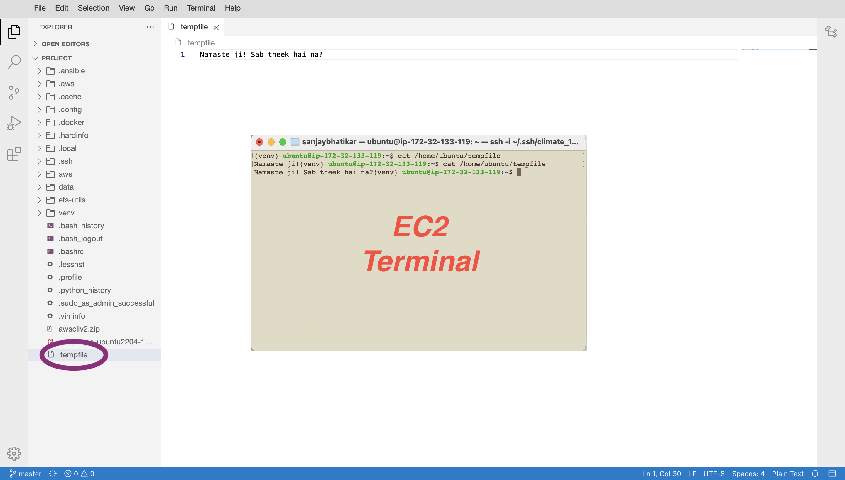
A tempfile
was created using the IDE with content “Namaste ji!”. The changes were verified using cat \home\ubuntu\templfile
on the host instance. Then the contents of the file were modified and changes verified. With this validation of the approach to fix the permissions error, the final docker run
command was as follows:
docker run --init \
--name theia_service \
--restart always \
-d -p 3030:3000 \
-v /home/ubuntu/:/home/project \
-u $(id -u ubuntu):$(id -g ubuntu) \
t1m0thyj/theia-alpine
Going headless doesn’t mean having to forgo an IDE. With Docker, the installation process can be painless and fruitful.
Join our FastAI class to learn from experienced instructors who excel not only in building state-of-the-art models but also in tackling complex engineering challenges in real-world scenarios. Our instructors bring a wealth of expertise from successfully deploying applications that solve tangible problems and reach customers effectively. Through hands-on projects and personalized guidance, you’ll gain practical skills in AI and machine learning, ensuring you’re equipped to create impactful solutions in your career. Whether you’re aiming to advance your knowledge or pivot into a new field, our FastAI class offers the perfect blend of theoretical foundations and real-world application to help you succeed.
SQL is described as a primitive programming language. The vocabulary of SQL, while compact, can still work wonders to shape data into a suitable form for visualization. One has only to be creative! Here is an example!
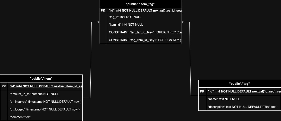
I have an app that records daily expenses. The Postgres DB saves each expense as a line item with the amount and date-time. Further, the expense is annotated with tags in key-value form to describe WHY (purpose of the expense), WHO (vendor engaged), WHERE (transaction location), etc.
I wanted two visualizations as follows:
DB Schema for Expense Tracking:
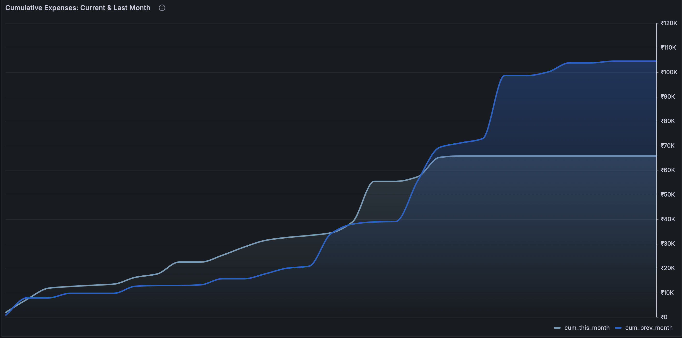
Cumulative Expenses:
The visualization requires a table with 31 rows for the days of the month and a column with cumulative expenses for current month and another column with the same data for the previous month.
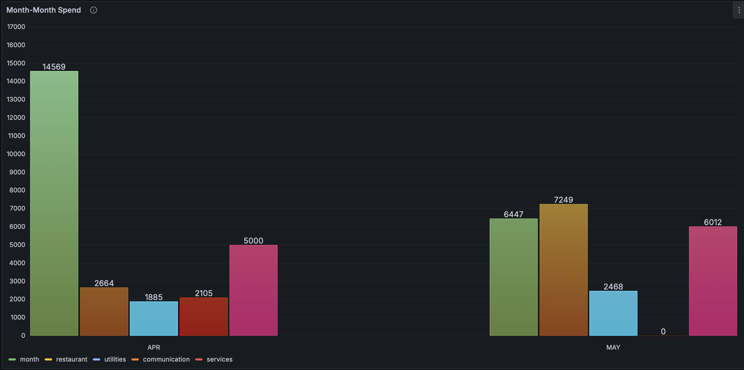
Categorical Expenses:
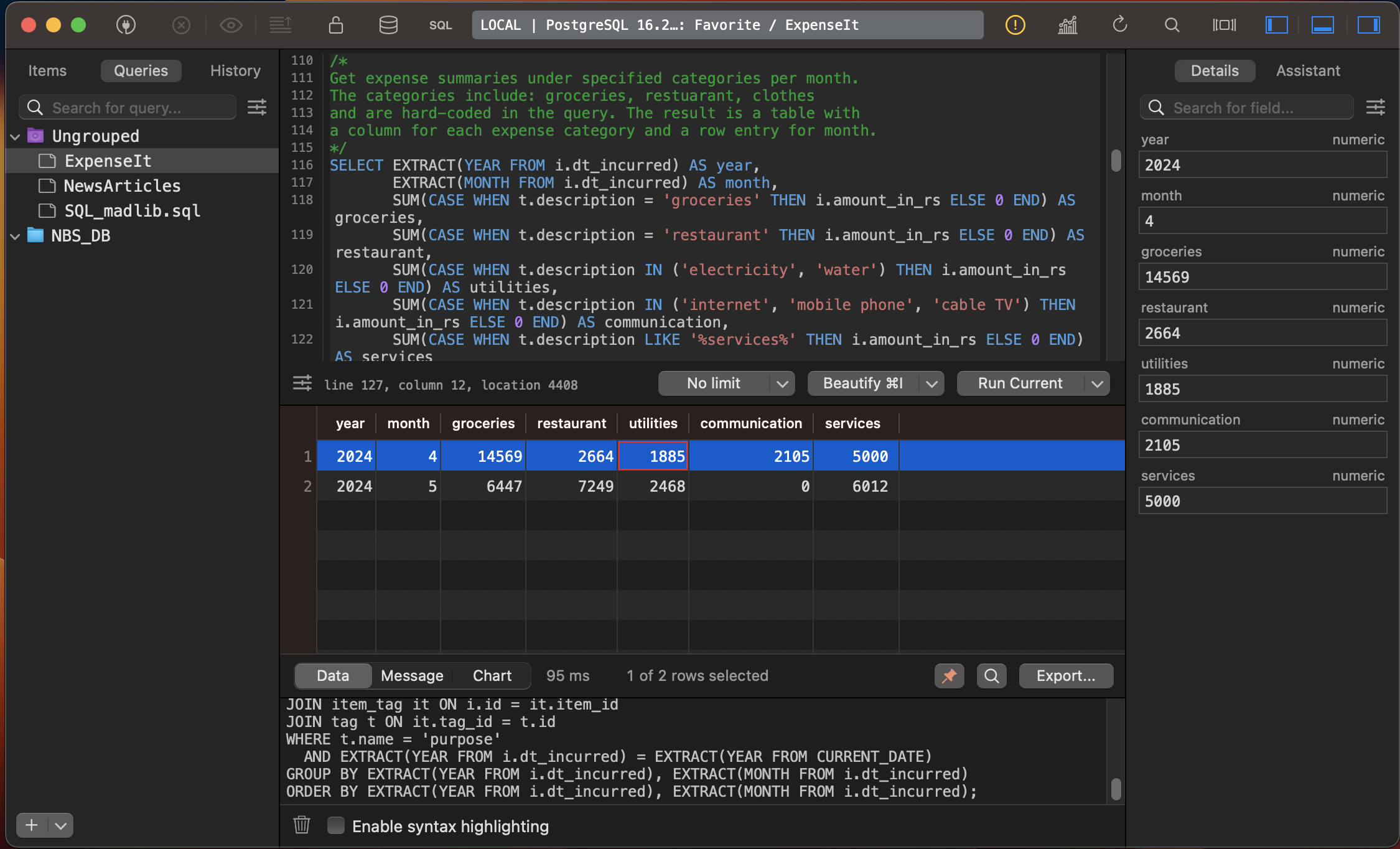
The visualization requires a table with a row for each month to be shown (2 months in the illustration – March, April) and one column for each category in which expenses are summarized.
Here is the query for the expense summaries by category for each month.
SELECT EXTRACT(YEAR FROM i.dt_incurred) AS year,
EXTRACT(MONTH FROM i.dt_incurred) AS month,
SUM(CASE WHEN t.description = 'groceries' THEN i.amount_in_rs ELSE 0 END) AS groceries,
SUM(CASE WHEN t.description = 'restaurant' THEN i.amount_in_rs ELSE 0 END) AS restaurant,
SUM(CASE WHEN t.description IN ('electricity', 'water') THEN i.amount_in_rs ELSE 0 END) AS utilities,
SUM(CASE WHEN t.description IN ('internet', 'mobile phone', 'cable TV') THEN i.amount_in_rs ELSE 0 END) AS communication,
SUM(CASE WHEN t.description LIKE '%services%' THEN i.amount_in_rs ELSE 0 END) AS services
FROM item i
JOIN item_tag it ON i.id = it.item_id
JOIN tag t ON it.tag_id = t.id
WHERE t.name = 'purpose'
AND EXTRACT(YEAR FROM i.dt_incurred) = EXTRACT(YEAR FROM CURRENT_DATE)
GROUP BY EXTRACT(YEAR FROM i.dt_incurred), EXTRACT(MONTH FROM i.dt_incurred)
ORDER BY EXTRACT(YEAR FROM i.dt_incurred), EXTRACT(MONTH FROM i.dt_incurred);
This produces the desired table as shown in the figure below.
We can understand this query with a simpler version that takes only one category to summarize expenses in current month.
SELECT SUM(i.amount_in_rs) AS total_amount
FROM item i
JOIN item_tag it ON i.id = it.item_id
JOIN tag t ON it.tag_id = t.id
WHERE t.name = 'purpose'
AND t.description = 'clothes'
AND EXTRACT(MONTH FROM i.dt_incurred) = EXTRACT(MONTH FROM CURRENT_DATE)
AND EXTRACT(YEAR FROM i.dt_incurred) = EXTRACT(YEAR FROM CURRENT_DATE);
The code allows only the current month and year and then selects rows tagged with ‘purpose’ as ‘clothes’. In the final version, we work off the same JOIN and add heft to the query to generate summaries in multiple categories of interest for each month. This is a variation on the Split-Apply-Combine strategy for Data Analysis, where you break up a big problem into manageable pieces, operate on each piece independently and then put all the pieces back together.
The main query builds on this to generate the categorical summaries of each month in the current year that data are available for!
Here is the query for cumulative sum.
WITH days AS (
SELECT generate_series(1, 31) AS day_of_month
),
current_month_expenses_by_day AS (
SELECT
EXTRACT(DAY FROM dt_incurred) AS day_of_month,
SUM(amount_in_rs) AS daily_expense
FROM item
WHERE EXTRACT(YEAR FROM dt_incurred) = EXTRACT(YEAR FROM CURRENT_DATE)
AND EXTRACT(MONTH FROM dt_incurred) = EXTRACT(MONTH FROM CURRENT_DATE)
GROUP BY EXTRACT(DAY FROM dt_incurred)
),
previous_month_expenses_by_day AS (
SELECT
EXTRACT(DAY FROM dt_incurred) AS day_of_month,
SUM(amount_in_rs) AS daily_expense
FROM item
WHERE EXTRACT(YEAR FROM dt_incurred) = EXTRACT(YEAR FROM CURRENT_DATE - INTERVAL '1 month')
AND EXTRACT(MONTH FROM dt_incurred) = EXTRACT(MONTH FROM CURRENT_DATE - INTERVAL '1 month')
GROUP BY EXTRACT(DAY FROM dt_incurred)
),
current_month_cumulative_expenses AS (
SELECT
d.day_of_month,
COALESCE(e.daily_expense, 0) AS daily_expense
FROM
days d
LEFT JOIN current_month_expenses_by_day e ON d.day_of_month = e.day_of_month
),
previous_month_cumulative_expenses AS (
SELECT
d.day_of_month,
COALESCE(e.daily_expense, 0) AS daily_expense
FROM
days d
LEFT JOIN previous_month_expenses_by_day e ON d.day_of_month = e.day_of_month
)
SELECT
d.day_of_month,
SUM(c.daily_expense) OVER (ORDER BY d.day_of_month) AS cum_this_month,
SUM(p.daily_expense) OVER (ORDER BY d.day_of_month) AS cum_prev_month
FROM
days d
LEFT JOIN current_month_cumulative_expenses c ON d.day_of_month = c.day_of_month
LEFT JOIN previous_month_cumulative_expenses p ON d.day_of_month = p.day_of_month
ORDER BY
d.day_of_month;
It is easier to understand cumulative summation in SQL with a simpler example.
Example to Illustrate:
Assume we have the following table @t:
id | SomeNumt |
---|---|
1 | 10 |
2 | 20 |
3 | 30 |
4 | 40 |
The query to add a column containing the cumulative sum is as follows:
select
t1.id,
t1.SomeNumt,
SUM(t2.SomeNumt) as sum
from
@t t1
inner join
@t t2
on t1.id >= t2.id
group by
t1.id,
t1.SomeNumt
order by
t1.id;
@t
is given aliases t1
and t2
to allow for a self-join. This is necessary to compare rows within the same table.inner join @t t2 on t1.id >= t2.id
t1.id >= t2.id
ensures that for each row in t1
, it will match with all rows in t2
where t2.id
is less than or equal to t1.id
. This effectively creates pairs of rows where each row in t1
will pair with all preceding rows in t2
including itself.Join Result:
The self-join on id
with the condition t1.id >= t2.id
will produce:
t1.id | t1.SomeNumt | t2.id | t2.SomeNumt |
---|---|---|---|
1 | 10 | 1 | 10 |
2 | 20 | 1 | 10 |
2 | 20 | 2 | 20 |
3 | 30 | 1 | 10 |
3 | 30 | 2 | 20 |
3 | 30 | 3 | 30 |
4 | 40 | 1 | 10 |
4 | 40 | 2 | 20 |
4 | 40 | 3 | 30 |
4 | 40 | 4 | 40 |
group by t1.id, t1.SomeNumt
t1.id
and t1.SomeNumt
. This ensures that we calculate the cumulative sum for each id
in t1
.SUM(t2.SomeNumt) as sum
id
from t1
), the query calculates the sum of SomeNumt
from all the rows in t2
that are less than or equal to the current id
in t1
. This effectively gives us the cumulative sum up to the current id
.Grouping and Summing Result:
Grouping by t1.id
and t1.SomeNumt
and summing t2.SomeNumt
:
t1.id | t1.SomeNumt | SUM(t2.SomeNumt) |
---|---|---|
1 | 10 | 10 |
2 | 20 | 30 |
3 | 30 | 60 |
4 | 40 | 100 |
This result shows the cumulative sum of SomeNumt
up to each id
. We have thus found a method of taking cumulative sum in SQL.
Recap:
id
in t1
, the join finds all preceding rows including itself in t2
.sum
function then calculates the total of SomeNumt
for these rows.id
in t1
.SomeNumt
for each id
, effectively showing how the sum accumulates as id
increases.While this is a clever solution, it has a downside that the operation has O(n^2) complexity. So the computational effort explodes exponentially. When our table grows to a million rows, we need a different approach!
SELECT
id,
SomeNumt,
SUM(SomeNumt) OVER (ORDER BY id) AS cumulative_sum
FROM
@t
ORDER BY
id;
Optimized Query:
The optimized query uses the SUM OVER
window function:
SUM(SomeNumt) OVER (ORDER BY id)
calculates a running total (cumulative sum) of SomeNumt
values in the order of id
.Window functions perform a calculation across a set of table rows that are somehow related to the current row. Unlike aggregate functions, window functions do not cause rows to become grouped into a single output row.
How SUM OVER
Works:
ORDER BY
Clause: The ORDER BY id
inside the OVER
clause specifies the order in which the rows are processed for the sum.SUM(SomeNumt) OVER (ORDER BY id)
computes the cumulative sum by adding the current row’s SomeNumt
to the sum of all previous rows’ SomeNumt
.Efficiency Gains: O(n) Complexity: The window function computes the cumulative sum in a single pass through the data, making it O(n) in complexity, significantly improving performance over the O(n^2) complexity of the self-join.
Here, then, is how we query the cumulative expense over days of the current month.
/*
Get cumulative expense by day of the month for current month.
*/
WITH days AS (
SELECT generate_series(1, 31) AS day_of_month
),
expenses_by_day AS (
SELECT
EXTRACT(DAY FROM dt_incurred) AS day_of_month,
SUM(amount_in_rs) AS daily_expense
FROM item
WHERE DATE_TRUNC('month', dt_incurred) = DATE_TRUNC('month', CURRENT_DATE)
GROUP BY EXTRACT(DAY FROM dt_incurred)
),
cumulative_expenses AS (
SELECT
d.day_of_month,
COALESCE(e.daily_expense, 0) AS daily_expense
FROM
days d
LEFT JOIN expenses_by_day e ON d.day_of_month = e.day_of_month
)
SELECT
day_of_month,
SUM(daily_expense) OVER (ORDER BY day_of_month) AS cum_this_month
FROM
cumulative_expenses
ORDER BY
day_of_month;
Here is how it works:
WITH days AS (
SELECT generate_series(1, 31) AS day_of_month
)
expenses_by_day AS (
SELECT
EXTRACT(DAY FROM dt_incurred) AS day_of_month,
SUM(amount_in_rs) AS daily_expense
FROM item
WHERE DATE_TRUNC('month', dt_incurred) = DATE_TRUNC('month', CURRENT_DATE)
GROUP BY EXTRACT(DAY FROM dt_incurred)
)
dt_incurred
column and summing the amount_in_rs
.
cumulative_expenses AS (
SELECT
d.day_of_month,
COALESCE(e.daily_expense, 0) AS daily_expense
FROM
days d
LEFT JOIN expenses_by_day e ON d.day_of_month = e.day_of_month
)
SELECT
day_of_month,
SUM(daily_expense) OVER (ORDER BY day_of_month) AS cum_this_month
FROM
cumulative_expenses
ORDER BY
day_of_month;
The main query builds on this to calculate the cumulative expenses for the previous month in addition to the current month.
SQL is a technology that is easy to underestimate in the Age of AI, but we do so at our own peril. Particularly when building data pipelines, one can use SQL to reshape data into the form suitable for consumption at the end-point – or as close to it as possible. In the use-case of expense reporting, SQL opened to door to compelling visualizations using templates in Grafana.
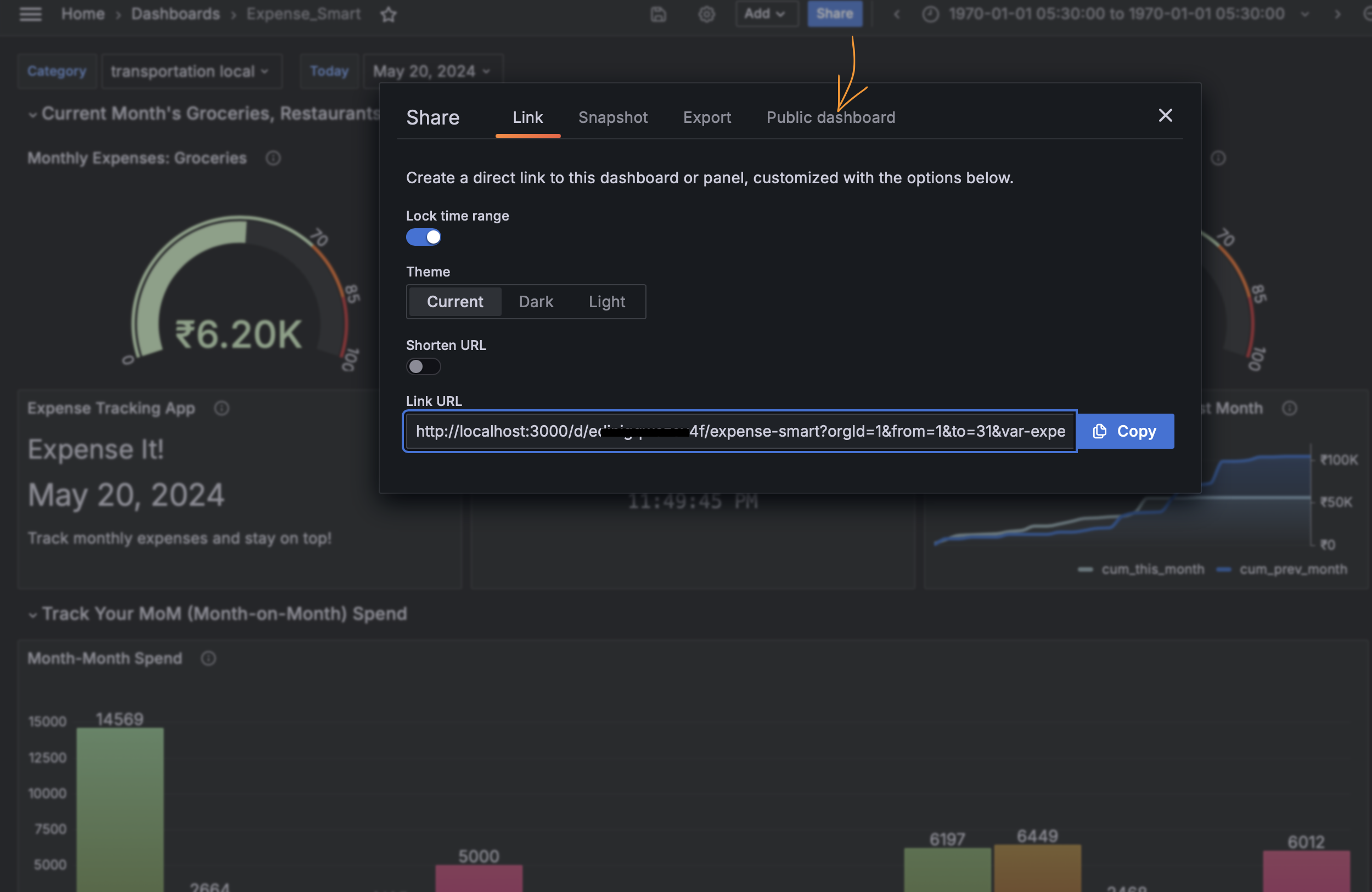
Looking to elevate your AI skills? Join our FastAI course! We cover not only cutting-edge modeling techniques but also the essential skills for acquiring, managing, and visualizing data. Learn from Ph.D. instructors who guide you through the entire process, from data collection to impactful visualizations, ensuring you’re equipped to tackle real-world challenges.
Building Machine Learning or AI models is just the beginning. Conveying the insights derived from these models is equally, if not more, important. Interactive visualizations are powerful tools for gaining buy-in and influencing decisions. However, creating effective visualizations can often require as much effort as the modeling itself.
Use Grafana in Docker on Raspberry Pi
Grafana offers a low-code or no-code solution for creating dashboards. By connecting queries to your data backend, you can quickly develop visualization templates with live data feeds. Grafana enables you to generate compelling visualizations and craft a narrative that supports your recommended actions. For example, you can use gauges to track monthly spending against a budget and recommend cost-saving measures like eating in instead of dining out.
ollow these steps to set up Grafana on your Raspberry Pi:
docker pull grafana/grafana
chown 472:472 /path/to/grafana/data
.
docker run --name grafana_service \
--restart always \
-d -p 3000:3000 \
-v /path/to/grafana/data:/var/lib/grafana \
-v /path/to/grafana/provisioning:/etc/grafana/provisioning \
-e GF_SECURITY_ADMIN_USER=admin \
-e GF_SECURITY_ADMIN_PASSWORD=topsecretphrase \
grafana/grafana
his command creates a Docker container named grafana_service with persistent data storage in shared volumes and sets up an admin account.
To share your Grafana dashboards:
By following these steps, you can effectively share your Grafana dashboards, ensuring that your visualizations reach your intended audience.
With Grafana and Docker, setting up and sharing interactive visualizations on your Raspberry Pi has never been easier. Use these tools to create compelling dashboards that effectively communicate your data insights.
Join our FastAI class to master not only the art of building robust AI models but also the essential skills of visualizing results and deploying software seamlessly into the hands of customers. Our course, led by experienced Ph.D. instructors, covers the full spectrum of AI development—from crafting accurate models to creating interactive visualizations with tools like Grafana and managing deployments using Docker on platforms like Raspberry Pi. Gain the comprehensive expertise needed to turn data into actionable insights and deliver real-world applications efficiently.
Docker is addictive. As it becomes an indispensable tool in our toolkit, we need a way to streamline container management. Docker offers Docker Desktop, a GUI application, for Mac and Windows users. For Raspberry Pi, I recommend Portainer.
Portainer provides an intuitive web-based interface to manage Docker containers, making it easy to start, stop, modify, or remove containers and monitor usage statistics. It runs in its own container and is well-suited for single-board computers (SBCs) like the Raspberry Pi running Raspbian.
Here’s how to get Portainer up and running on your Raspberry Pi:
docker pull portainer/linux-arm
docker run
command like so:
docker run --name portainer_service --network docker-net \
-d -p 9000:9000 \
-v /var/run/docker.sock:/var/run/docker.sock \
-v ~/Your/path/to/data:/data \
portainer/portainer:linux-arm
Now access Portainer from: http://localhost:9000. That is it!
Deploying AI Models in Real-World Situations
Being an AI practitioner means not only building models but also being familiar with various environments in which these models are deployed. Field applications often leverage platforms such as SBCs. The Raspberry Pi is a popular SBC that runs Linux and integrates seamlessly with various sensors and actuators.
In our FastAI course, you’ll learn from Ph.D. instructors who have invaluable expertise in both model building and the engineering required to deploy these models in real-world situations. We cover essential tools like Docker and Portainer, equipping you with the skills needed to put your AI applications into the hands of users effectively.
Join us to bridge the gap between developing AI models and deploying them in practical environments.
In an earlier blogpost, we looked at why Docker is such an indispensable tool in the developer or data scientist’s toolkit, especially for shipping code that runs consistently across different environments. The Raspberry Pi, with its ARM architecture, provides a great example. Running software developed in traditional x86 environments on the Raspberry Pi can be challenging. Docker helps surmount these challenges and saves us endless frustration.
I recently built an app for tracking expenses, particularly when my kid spent too much money on Zomato, a food delivery app! The idea was to set a monthly budget and track expenses against it. Visualizing data is crucial for self-adjustment on the path to improvement. The expense tracking system I built allows tracking expenses in common categories such as groceries, restaurants, utilities, etc.
I developed the app in the Python programming language. The app’s GUI, built in PyQt6, supports CRUD operations on a Postgres database. Users can create, view, update, and delete expenses. The architecture is a standard MVC framework with Pydantic business objects and SQLAlchemy ORM.
Additionally, I built a dashboard in Grafana, a browser-based dashboarding tool. I developed the app on my MacBook and deployed it on the “always on” Raspberry Pi 400 at home.
I encountered many hurdles when porting code to the Raspberry Pi. The PyQt6 library couldn’t be installed in a virtual environment using the pip installer, so I installed it system-wide from the Debian repository. This prevented running my Python code in the virtual environment. Consequently, other dependencies like Pydantic and SQLAlchemy also had to be installed system-wide.
I pulled the official Docker image for Postgres to get the database running. See this blogpost. However, finding a suitable SQL client was surprisingly difficult. I tried TablePlus, DBeaver, and Pgdmin, but each had issues post-installation, rendering them unusable.
A bad workman always blames his tools. Was I using the wrong tools or is the Raspberry Pi just Rubbish Pi?
The Raspberry Pi, being resource-constrained compared to a desktop, poses challenges in installing and running software. Docker can be invaluable in such situations. I was already running Postgres in a Docker container on the Raspberry Pi and found ARM-compatible containers for Pgadmin and Grafana. The pgAdmin container, provided by Elestio, is available as elestio/pgadmin.
Here’s how to install it:
docker pull elestio/pgadmin
Run the container:
docker run --name pgadmin_service \
-d -p 8080:8080 \
--network docker-net \
-e PGADMIN_DEFAULT_EMAIL=handsomest.coder@email.com \
-e PGADMIN_DEFAULT_PASSWORD=topsecret \
-e PGADMIN_LISTEN_PORT=8080 \
-v ~/path/to/pgadmin/servers.json:/pgadmin4/servers.json \
elestio/pgadmin
This command starts a Pgadmin container named pgadmin_service
in the background, accessible via http://localhost:8080
, connected to the docker-net
network, using the specified email and password for initial login credentials, and mounting a servers.json
file for predefined server connections.
Using Docker images for Pgadmin and Postgres provided a smooth path to setting up these vital data assets on my Raspberry Pi. This approach should generally be the default for installing software in app development. For example, when building home automation systems, it’s beneficial to containerize services like Mosquito MQTT, Node-Red, InfluxDB, and Grafana that are part of developer’s IoT stack. Refer to this YouTube video for a guide. For managing all these containers with a graphical UI, use Portainer, available as a free community edition from Docker.
Unlock the full potential of AI with our FastAI course, where you’ll not only master AI integration into applications but also gain essential skills like Docker, crucial for deploying and managing your apps in real-world environments. Learn to bridge the gap between development and practical implementation, ensuring your AI solutions are robust, scalable, and ready for end-users. Join us to transform your technical expertise into powerful, customer-ready applications.
Back in the day, when I wrote apps in C/C++, I compiled the code into an executable for shipping. When we code in Python, how do we ship code?
We could simply send our code to the customer to run it on their machine. But the environment in which our code would run at the customer’s end would almost never be identical to ours. Small differences in environment could mean our code doesn’t run and debugging such issues is a colossal waste of time, not to mention repeating the process for every customer.
But there is a better way and that is Docker!
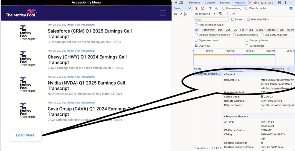
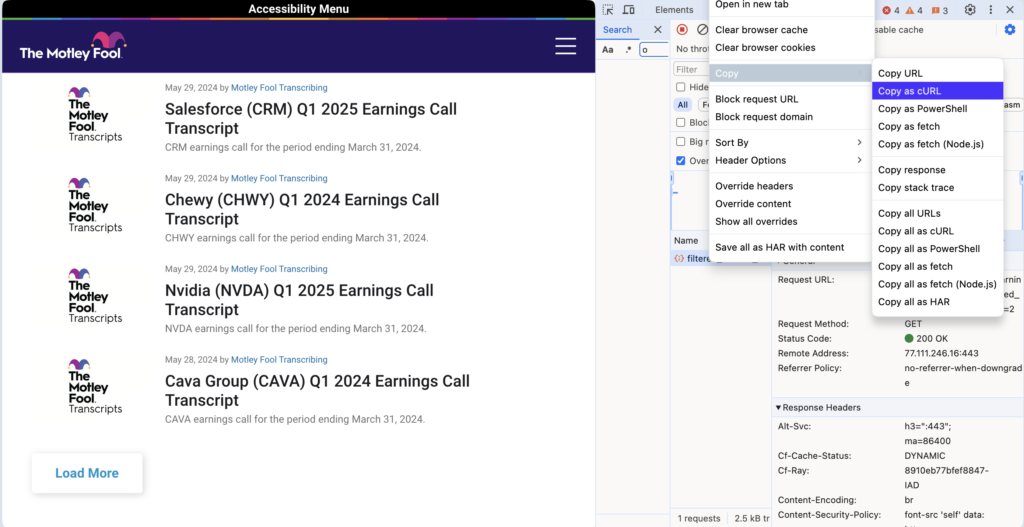
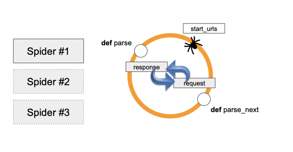
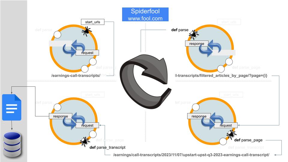
Here is a microservice I built that was part of a larger app. It has a spider that crawls multiple web domains for content that it scrapes and puts into a Postgres warehouse. I built out the spider in Scrapy framework in Python 3 and used the psycopg2 client for database CRUD operations.
Shipping the code means replicating the environment on the machine where it will run. In the process, small changes may creep up. The version of Python or its dependencies may differ. The version of Postgres may also differ. The devil lies in details! Small differences can throw a spanner in the works. That is why, shipping code in this manner is not recommended.
Instead, dockerize the app!
Let’s start by dockerizing the Postgres warehouse. The steps are pulling the docker image from docker hub and then spinning up the container!
Pull the image like so: docker pull postgres
Then spin up the container like so: docker run --name postgres_service --network scrappy-net -e POSTGRES_PASSWORD=topsecretpassword -d -p 5432:5432 -v /Your/path/to/volume:/var/lib/postgresql/data postgres
This command not only launches the container but also connects it to the Docker network for seamless communication among containers. (Refer this blogpost.) Additionally, it ensures data persistence by sharing a folder between the host machine and the container.
Let’s break down the docker run
command into its constituent parts:
docker run
: This is the command used to create and start a new container based on a specified image.--name postgres_service
: This flag specifies the name of the container. In this case, the container will be named “postgres_service”.--network scrappy-net
: This flag specifies the network that the container should connect to. In this case, the container will connect to the network named “scrappy-net”.-e POSTGRES_PASSWORD=topsecretpassword
: This flag sets an environment variable within the container. Specifically, it sets the environment variable POSTGRES_PASSWORD
to the value topsecretpassword
. This is typically used to configure the containerized application.-d
: This flag tells Docker to run the container in detached mode, meaning it will run in the background and won’t occupy the current terminal session.-p 5432:5432
: This flag specifies port mapping, binding port 5432 on the host machine to port 5432 in the container. Port 5432 is the default port used by PostgreSQL, so this allows communication between the host and the PostgreSQL service running inside the container.-v /Your/path/to/volume:/var/lib/postgresql/data
: This flag specifies volume mapping, creating a persistent storage volume for the PostgreSQL data. The format is -v <host-path>:<container-path>
. In this case, it maps a directory on the host machine (specified by /Your/path/to/volume
) to the directory inside the container where PostgreSQL stores its data (/var/lib/postgresql/data
). This ensures that the data persists even if the container is stopped or removed.postgres
: Finally, postgres
specifies the Docker image to be used for creating the container. In this case, it indicates that the container will be based on the official PostgreSQL image from Docker Hub.For creating a container from own code – Python scripts and dependencies, there are a few steps. The first step is creating a dockerfile. The dockerfile for our Scrapy app looks like so:
# Use the official Python 3.9 image
FROM python:3.9
# Set the working directory in the container
WORKDIR /app
# Copy the current directory contents into the container at /app
COPY . /app
# Install required dependencies
RUN pip install --no-cache-dir -r requirements.txt
# Set the entry point command for running the Scrapy spider
ENTRYPOINT ["scrapy", "crawl", "spidermoney"]
This Dockerfile automates the process of building the image and running the container. It ensures that the container has all the necessary dependencies to execute the Python app.
Let’s break down each line of the Dockerfile:
FROM python:3.9
: This instruction specifies the base image to build upon. It tells Docker to pull the Python 3.9 image from the Docker Hub registry. This image will serve as the foundation for our custom image.WORKDIR /app
: This instruction sets the working directory inside the container to /app
. This is where subsequent commands will be executed, and it ensures that any files or commands are relative to this directory.COPY . /app
: This instruction copies the contents of the current directory on the host machine (the directory where the Dockerfile is located) into the /app
directory within the container. It is a common practice to place the dockerfile in the project directory at the top level, for including application code and files inside the Docker image.RUN pip install --no-cache-dir -r requirements.txt
: This instruction runs the pip install
command inside the container to install the Python dependencies listed in the requirements.txt
file. The --no-cache-dir
flag ensures that pip doesn’t use any cache when installing packages, which can help keep the Docker image smaller.ENTRYPOINT ["scrapy", "crawl", "spidermoney"]
: This instruction sets the default command to be executed when the container starts. It specifies that the scrapy crawl spidermoney
command should be run. This command tells Scrapy, a web crawling framework, to execute a spider named “spidermoney”. When the container is launched, it will automatically start executing this command, running the Scrapy spider.
The dockerfile is a recipe. The steps to prepare the dish are as follows:
docker build -t scrapy-app .
. The dockerfile is a series of instructions to build a docker image from. The build process downloads the base layer and adds a layer with every instruction. Thus, layer by layer, a new image in constructed which has everything needed to spin up a container that runs the app.docker run
command. For example: docker run --name scrapy_service --network scrappy-net -e DB_HOST=postgres_service scrapy-app
. This command creates container named ‘scrapy_service’ from the image ‘scrapy-app’ and connects it to the network ‘scrappy-net’. The name of the container running Postgres is passed as an environment variable with -e
flag to configure the app to work with the database instance.Once the microservice is containerized, launching it is as simple as starting the containers. Start the Postgres container first, followed by the app container. This can be easily done from the Docker dashboard.
Verifying Deployment:
Verify the results by examining the Postgres database before and after running the microservice. Running SQL queries can confirm that the spider has successfully crawled web domains and added new records to the database.
The figures show that 1232 records were added in this instance.
Now shipping the code is as simple as docker push
to post the images to docker hub followed by docker pull
on the target machine.
With Docker, shipping code becomes a streamlined process. Docker encapsulates applications and their dependencies, ensuring consistency across different environments. By containerizing both the database and the Python app, we simplify deployment and guarantee reproducibility, ultimately saving time and effort.
In conclusion, Docker revolutionizes the way we ship and deploy code, making it an indispensable tool for modern software development.
Being in the AI profession is more than just coding neural networks. Getting them into the hands of customers demands a thorough understanding of contemporary microservices architecture patterns. Learn from experienced instructors who can be your guide through our comprehensive coaching program powered by FastAI. Gain insights into cutting-edge techniques and best practices for building AI applications that not only meet the demands of today’s market but also seamlessly integrate into existing systems. From understanding advanced algorithms to mastering deployment strategies, our Ph.D. instructors will equip you with the skills and knowledge needed to succeed in the dynamic world of AI deployment. Join us and take your AI career to new heights with hands-on training and personalized guidance.
It is vital for a company to continuously monitor the changing business landscape for both threats and opportunities. This critical function involves prospecting opportunities and gathering intelligence on competitors, which is then synthesized by analysts into executive briefs with actionable recommendations. This task entails sifting through a wide array of information from diverse sources such as websites, regulatory filings, social media, and news articles, contributed by journalists, analysts, influencers, regulators, as well as internal company staff and officers. Automation efforts have often focused on casting a wider net, resulting in more pressure on downstream analysis and insight generation where the value lies. Recent rapid developments in Generative AI and the emergence of Large Language Models (LLMs) in Open Source have opened the door to automation of these downstream activities. In particular, the “co-pilot” mode of assistive AI offers the potential to increase productivity and reduce the risk of missed opportunities. We built a chatbot assistant in one such use-case for Bayer Crop Science USA.
The challenges of automating information digestion for insight generation can be distilled into two key problems: retrieving relevant information from a large corpus and using that information to contextualize responses. To address the first challenge, we employed Semantic Search, which allows natural language queries to be posed to a large text corpus, yielding ranked results. For the second challenge, we adopted Retrieval Augmented Generation (RAG), a technique that leverages Semantic Search results to provide transient context to a pre-trained Large Language Model (LLM) like ChatGPT. This approach avoids the computational intensity of fine-tuning LLMs and ensures that responses are guided by recent and relevant information without permanently embedding it into the neural network.
Retrieval Augmented Generation (RAG) utilizes text retrieved by Semantic Search to augment a Large Language Model’s response to a prompt. Semantic Search employs embeddings, which represent text in a vector space. We implemented Semantic Search using the nomic-embed-text model within the ollama framework with Chroma as vector store. We wrapped a Streamlit UI around the vector store to enable search in a “standalone” mode. We used the LangChain framework to pull together the Retrieval Augmented Generation (RAG) workflow, with the Llama2 LLM from Meta with 13B parameters. The user’s prompt is routed to the Semantic Search engine to retrieve relevant documents, which then serve as context for the LLM to use in responding. This approach enhances the LLM’s ability to provide informed responses, effectively supporting the team’s work. The system has been lauded by users at Bayer Crop Science USA, who appreciate its capacity to provide tailored insights and streamline decision-making processes.
Empower yourself with the transformative capabilities of Deep Learning AI through our comprehensive coaching program centered on FastAI. Dive deep into the intricacies of AI and emerge equipped with invaluable skills in natural language processing, computer vision, and beyond. Our hands-on approach ensures that learners of all levels, from beginners to seasoned practitioners, grasp complex concepts with ease and confidence. Join us on a journey of discovery and mastery, where cutting-edge knowledge meets practical application, propelling you towards success in the dynamic world of AI.
In the realm of Biotech R&D, the cultivation of genetically engineered plants through tissue culture stands as a pivotal process, deviating from traditional seed-based methods to derive plants from embryos. Particularly in the case of corn, this intricate procedure spans 7-9 weeks, commencing with the manipulation of embryonic tissue, deliberately injured and exposed to agrobacterium tumefaciens, a specific bacteria facilitating DNA transfer. The outcome manifests as plant transformation, marked by the integration of foreign genes into the targeted specimen. Notably, the success rates of this process are dismally low, with a meager 2% or fewer embryos evolving into viable plants boasting the intended genetics. Hence, it becomes imperative to discern the success or failure of plant transformation at the earliest stages.
Historically, this determination was only feasible at the culmination of the 7-9 week period when plantlets emerged. Consequently, more than 98% of non-transformable embryos occupied valuable laboratory space and consumed essential resources. Given that plant transformation transpires within specialized chambers, maintaining stringent environmental conditions (temperature, humidity, and light), the inefficient utilization of space becomes a bottleneck in the downstream biotech R&D pipeline. To address this challenge, we conceptualized and implemented a groundbreaking solution: a Convolutional Neural Network (CNN) designed to scrutinize embryos and identify non-transformable ones within the initial two weeks post the initiation of plant transformation. This computer vision solution revolutionized the traditional approach, facilitating early detection and removal of approximately half of the non-transformable embryos. This, in turn, averted the necessity for a capital expenditure ranging between $10-15 million to expand the facility, effectively enhancing throughput by 1.5 to 2 times. Technologically, our approach incorporated an ensemble of deep learning models, achieving an impressive performance with over 90% sensitivity at 70% specificity during testing.
Leveraging pre-trained models and neural transfer learning, we curated an extensive in-house dataset comprising 15,000 images meticulously labeled by cell biologists. These images, capturing various stages of embryonic development, were acquired using both an ordinary DSLR camera and a proprietary hyperspectral imaging robot. Our experimentation precisely determined the optimal timeframe for image acquisition post the initiation of plant transformation, establishing that images from a conventional DSLR were on par with those from the hyperspectral camera for the classification task. The impact of our work extends far beyond the confines of the laboratory, catalyzing a wave of innovations in computer vision within biotechnology R&D, spanning laboratories, greenhouses, and field applications. This progressive integration has not only optimized the R&D pipeline but has also significantly accelerated time-to-market, positioning our consultancy at the forefront of transformative advancements in the biotech sector
Interested in the power of deep learning to propel your Python skills to new heights? With our FastAI coaching, you will dive into the world of computer vision and other applications of deep learning. Our expertly crafted course is tailored for those with a minimum of one year of Python programming experience and taught by experienced Ph.D. instructors. FastAI places the transformative magic of deep learning directly into your hands. From day one, you’ll embark on a journey of practical application, building innovative apps and honing your Python proficiency along the way. Don’t just code —immerse yourself in the art and science of deep learning with FastAI.
Suppose I have two docker containers on a host machine- an app running in one container, requiring the use of database running in another container. The architecture is as shown in the figure.
In the figure, the Postgres container is named ‘postgres_service’ and is based on official postgres image on docker. The data reside on a shared volume with local host. In this way, data are persisted even after container is removed.
The app container is named ‘scrapy_service’ and is based on an image created starting from official Python 3.9 base image for linux. The application code implements a web-crawler that scrapes financial news websites.
The web-scraper puts data into the postgres database. How to access postgres?
On the host machine, the postgres service is accessible at ‘localhost’ on port 5432. However, this will not work from inside the app container where ‘localhost’ is self-referential.
Solution? We create a docker network and connect both containers to it.
Create docker network and connect postgres container to it. Inspect and verify.
Spin up app’s container with connection to the network.
docker create network scrappy-net
creates network named scrappy-net.docker network connect scrappy-net postgres_service
connects the (running) postgres container to the network.docker network inspect scrappy-net
shows the network and what’s on it. We now have a network ready to accept connections and exchange messages with other containers. Docker will do the DNS lookup with container name.
docker build -t scrapy-app .
builds the image named scrapy-app. The project directory must have dockerfile and requirements manifest. The entry-point that launches spider is scrapy crawl spidermoney
or scrapy crawl spidermint
.docker run –-name scrapy_service –-network scrappy-net -e DB_HOST=postgres_service scrapy-app
spins up the container with connection to the network. It launches the crawler as per the entry-point spec. The container exits when the job is done. Thereafter, it can be re-run as docker start scrapy_service
with persistent network connection.docker logs scrapy_service > /Users/sanjaybhatikar/Documents/tempt.txt 2>&1
saves the app’s strreamed output on stderr and stdout to temp text file for inspection.