Unlocking the Power of Language: Leveraging Large Language Models for Next-Gen Semantic Search and Real-World Applications
Invited talk at Calfus, Pune, June 20, 2024.
Back in the day, when I wrote apps in C/C++, I compiled the code into an executable for shipping. When we code in Python, how do we ship code?
We could simply send our code to the customer to run it on their machine. But the environment in which our code would run at the customer’s end would almost never be identical to ours. Small differences in environment could mean our code doesn’t run and debugging such issues is a colossal waste of time, not to mention repeating the process for every customer.
But there is a better way and that is Docker!
Here is a microservice I built that was part of a larger app. It has a spider that crawls multiple web domains for content that it scrapes and puts into a Postgres warehouse. I built out the spider in Scrapy framework in Python 3 and used the psycopg2 client for database CRUD operations.
Shipping the code means replicating the environment on the machine where it will run. In the process, small changes may creep up. The version of Python or its dependencies may differ. The version of Postgres may also differ. The devil lies in details! Small differences can throw a spanner in the works. That is why, shipping code in this manner is not recommended.
Instead, dockerize the app!
Let’s start by dockerizing the Postgres warehouse. The steps are pulling the docker image from docker hub and then spinning up the container!
Pull the image like so: docker pull postgres
Then spin up the container like so: docker run --name postgres_service --network scrappy-net -e POSTGRES_PASSWORD=topsecretpassword -d -p 5432:5432 -v /Your/path/to/volume:/var/lib/postgresql/data postgres
This command not only launches the container but also connects it to the Docker network for seamless communication among containers. (Refer this blogpost.) Additionally, it ensures data persistence by sharing a folder between the host machine and the container.
Let’s break down the docker run
command into its constituent parts:
docker run
: This is the command used to create and start a new container based on a specified image.--name postgres_service
: This flag specifies the name of the container. In this case, the container will be named “postgres_service”.--network scrappy-net
: This flag specifies the network that the container should connect to. In this case, the container will connect to the network named “scrappy-net”.-e POSTGRES_PASSWORD=topsecretpassword
: This flag sets an environment variable within the container. Specifically, it sets the environment variable POSTGRES_PASSWORD
to the value topsecretpassword
. This is typically used to configure the containerized application.-d
: This flag tells Docker to run the container in detached mode, meaning it will run in the background and won’t occupy the current terminal session.-p 5432:5432
: This flag specifies port mapping, binding port 5432 on the host machine to port 5432 in the container. Port 5432 is the default port used by PostgreSQL, so this allows communication between the host and the PostgreSQL service running inside the container.-v /Your/path/to/volume:/var/lib/postgresql/data
: This flag specifies volume mapping, creating a persistent storage volume for the PostgreSQL data. The format is -v <host-path>:<container-path>
. In this case, it maps a directory on the host machine (specified by /Your/path/to/volume
) to the directory inside the container where PostgreSQL stores its data (/var/lib/postgresql/data
). This ensures that the data persists even if the container is stopped or removed.postgres
: Finally, postgres
specifies the Docker image to be used for creating the container. In this case, it indicates that the container will be based on the official PostgreSQL image from Docker Hub.For creating a container from own code – Python scripts and dependencies, there are a few steps. The first step is creating a dockerfile. The dockerfile for our Scrapy app looks like so:
# Use the official Python 3.9 image
FROM python:3.9
# Set the working directory in the container
WORKDIR /app
# Copy the current directory contents into the container at /app
COPY . /app
# Install required dependencies
RUN pip install --no-cache-dir -r requirements.txt
# Set the entry point command for running the Scrapy spider
ENTRYPOINT ["scrapy", "crawl", "spidermoney"]
This Dockerfile automates the process of building the image and running the container. It ensures that the container has all the necessary dependencies to execute the Python app.
Let’s break down each line of the Dockerfile:
FROM python:3.9
: This instruction specifies the base image to build upon. It tells Docker to pull the Python 3.9 image from the Docker Hub registry. This image will serve as the foundation for our custom image.WORKDIR /app
: This instruction sets the working directory inside the container to /app
. This is where subsequent commands will be executed, and it ensures that any files or commands are relative to this directory.COPY . /app
: This instruction copies the contents of the current directory on the host machine (the directory where the Dockerfile is located) into the /app
directory within the container. It is a common practice to place the dockerfile in the project directory at the top level, for including application code and files inside the Docker image.RUN pip install --no-cache-dir -r requirements.txt
: This instruction runs the pip install
command inside the container to install the Python dependencies listed in the requirements.txt
file. The --no-cache-dir
flag ensures that pip doesn’t use any cache when installing packages, which can help keep the Docker image smaller.ENTRYPOINT ["scrapy", "crawl", "spidermoney"]
: This instruction sets the default command to be executed when the container starts. It specifies that the scrapy crawl spidermoney
command should be run. This command tells Scrapy, a web crawling framework, to execute a spider named “spidermoney”. When the container is launched, it will automatically start executing this command, running the Scrapy spider.
The dockerfile is a recipe. The steps to prepare the dish are as follows:
docker build -t scrapy-app .
. The dockerfile is a series of instructions to build a docker image from. The build process downloads the base layer and adds a layer with every instruction. Thus, layer by layer, a new image in constructed which has everything needed to spin up a container that runs the app.docker run
command. For example: docker run --name scrapy_service --network scrappy-net -e DB_HOST=postgres_service scrapy-app
. This command creates container named ‘scrapy_service’ from the image ‘scrapy-app’ and connects it to the network ‘scrappy-net’. The name of the container running Postgres is passed as an environment variable with -e
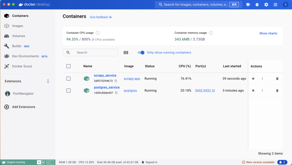
flag to configure the app to work with the database instance.Once the microservice is containerized, launching it is as simple as starting the containers. Start the Postgres container first, followed by the app container. This can be easily done from the Docker dashboard.
Verifying Deployment:
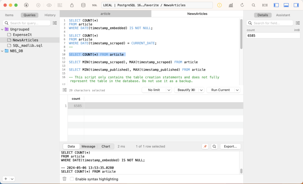
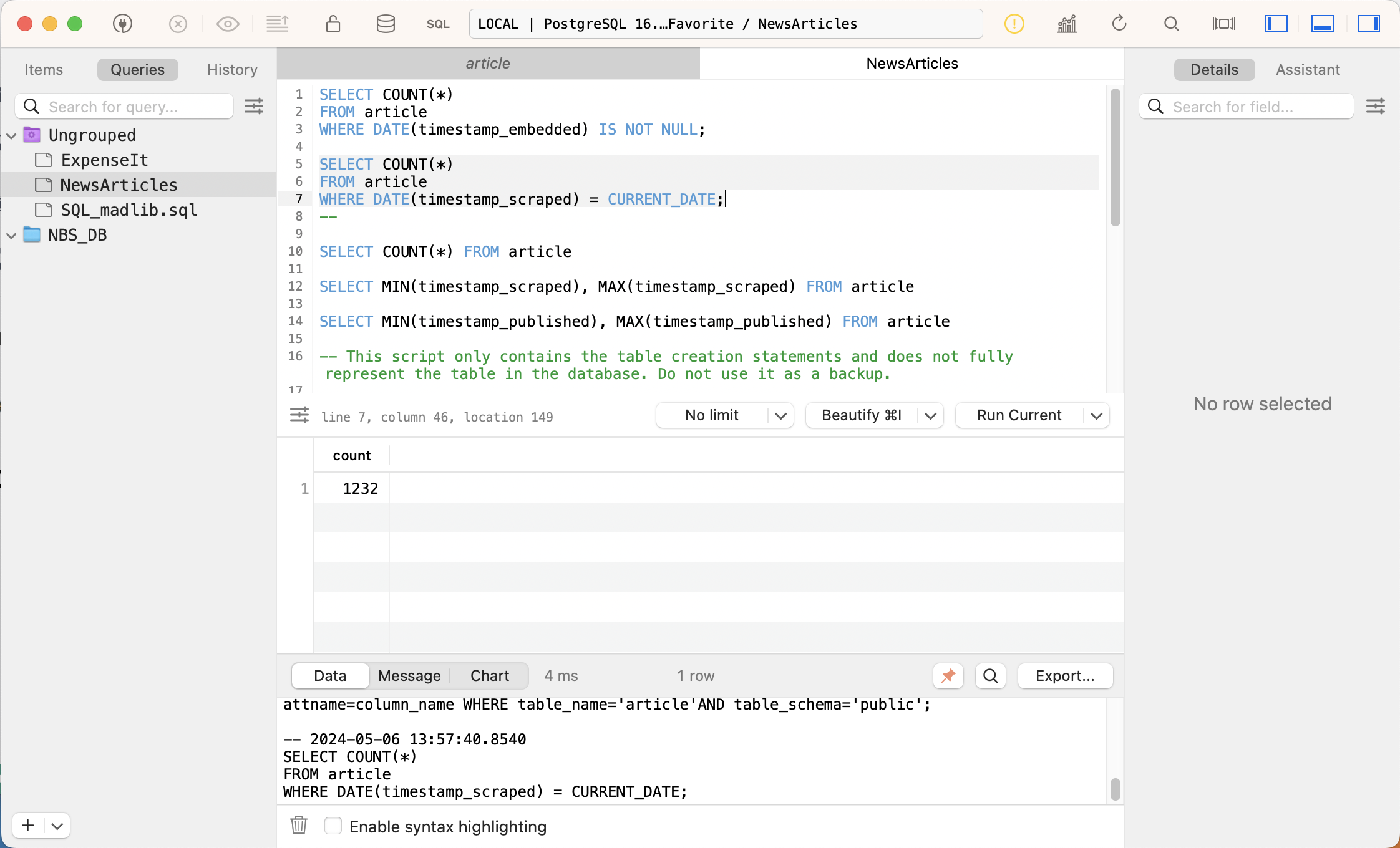
Verify the results by examining the Postgres database before and after running the microservice. Running SQL queries can confirm that the spider has successfully crawled web domains and added new records to the database.
The figures show that 1232 records were added in this instance.
Now shipping the code is as simple as docker push
to post the images to docker hub followed by docker pull
on the target machine.
With Docker, shipping code becomes a streamlined process. Docker encapsulates applications and their dependencies, ensuring consistency across different environments. By containerizing both the database and the Python app, we simplify deployment and guarantee reproducibility, ultimately saving time and effort.
In conclusion, Docker revolutionizes the way we ship and deploy code, making it an indispensable tool for modern software development.
Being in the AI profession is more than just coding neural networks. Getting them into the hands of customers demands a thorough understanding of contemporary microservices architecture patterns. Learn from experienced instructors who can be your guide through our comprehensive coaching program powered by FastAI. Gain insights into cutting-edge techniques and best practices for building AI applications that not only meet the demands of today’s market but also seamlessly integrate into existing systems. From understanding advanced algorithms to mastering deployment strategies, our Ph.D. instructors will equip you with the skills and knowledge needed to succeed in the dynamic world of AI deployment. Join us and take your AI career to new heights with hands-on training and personalized guidance.
In the realm of Biotech R&D, the cultivation of genetically engineered plants through tissue culture stands as a pivotal process, deviating from traditional seed-based methods to derive plants from embryos. Particularly in the case of corn, this intricate procedure spans 7-9 weeks, commencing with the manipulation of embryonic tissue, deliberately injured and exposed to agrobacterium tumefaciens, a specific bacteria facilitating DNA transfer. The outcome manifests as plant transformation, marked by the integration of foreign genes into the targeted specimen. Notably, the success rates of this process are dismally low, with a meager 2% or fewer embryos evolving into viable plants boasting the intended genetics. Hence, it becomes imperative to discern the success or failure of plant transformation at the earliest stages.
Historically, this determination was only feasible at the culmination of the 7-9 week period when plantlets emerged. Consequently, more than 98% of non-transformable embryos occupied valuable laboratory space and consumed essential resources. Given that plant transformation transpires within specialized chambers, maintaining stringent environmental conditions (temperature, humidity, and light), the inefficient utilization of space becomes a bottleneck in the downstream biotech R&D pipeline. To address this challenge, we conceptualized and implemented a groundbreaking solution: a Convolutional Neural Network (CNN) designed to scrutinize embryos and identify non-transformable ones within the initial two weeks post the initiation of plant transformation. This computer vision solution revolutionized the traditional approach, facilitating early detection and removal of approximately half of the non-transformable embryos. This, in turn, averted the necessity for a capital expenditure ranging between $10-15 million to expand the facility, effectively enhancing throughput by 1.5 to 2 times. Technologically, our approach incorporated an ensemble of deep learning models, achieving an impressive performance with over 90% sensitivity at 70% specificity during testing.
Leveraging pre-trained models and neural transfer learning, we curated an extensive in-house dataset comprising 15,000 images meticulously labeled by cell biologists. These images, capturing various stages of embryonic development, were acquired using both an ordinary DSLR camera and a proprietary hyperspectral imaging robot. Our experimentation precisely determined the optimal timeframe for image acquisition post the initiation of plant transformation, establishing that images from a conventional DSLR were on par with those from the hyperspectral camera for the classification task. The impact of our work extends far beyond the confines of the laboratory, catalyzing a wave of innovations in computer vision within biotechnology R&D, spanning laboratories, greenhouses, and field applications. This progressive integration has not only optimized the R&D pipeline but has also significantly accelerated time-to-market, positioning our consultancy at the forefront of transformative advancements in the biotech sector
Interested in the power of deep learning to propel your Python skills to new heights? With our FastAI coaching, you will dive into the world of computer vision and other applications of deep learning. Our expertly crafted course is tailored for those with a minimum of one year of Python programming experience and taught by experienced Ph.D. instructors. FastAI places the transformative magic of deep learning directly into your hands. From day one, you’ll embark on a journey of practical application, building innovative apps and honing your Python proficiency along the way. Don’t just code —immerse yourself in the art and science of deep learning with FastAI.
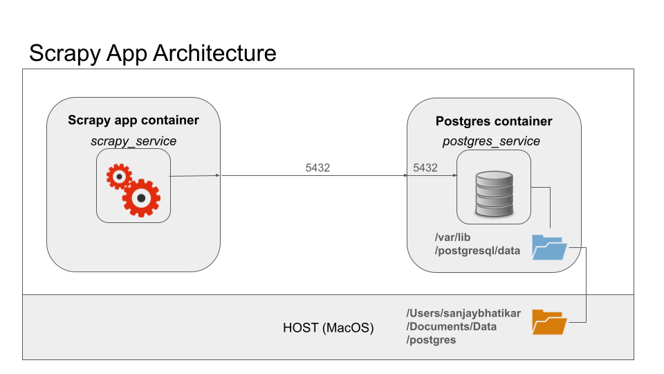
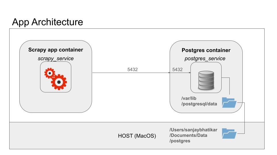
Suppose I have two docker containers on a host machine- an app running in one container, requiring the use of database running in another container. The architecture is as shown in the figure.
In the figure, the Postgres container is named ‘postgres_service’ and is based on official postgres image on docker. The data reside on a shared volume with local host. In this way, data are persisted even after container is removed.
The app container is named ‘scrapy_service’ and is based on an image created starting from official Python 3.9 base image for linux. The application code implements a web-crawler that scrapes financial news websites.
The web-scraper puts data into the postgres database. How to access postgres?
On the host machine, the postgres service is accessible at ‘localhost’ on port 5432. However, this will not work from inside the app container where ‘localhost’ is self-referential.
Solution? We create a docker network and connect both containers to it.
Create docker network and connect postgres container to it. Inspect and verify.
Spin up app’s container with connection to the network.
docker create network scrappy-net
creates network named scrappy-net.docker network connect scrappy-net postgres_service
connects the (running) postgres container to the network.docker network inspect scrappy-net
shows the network and what’s on it. We now have a network ready to accept connections and exchange messages with other containers. Docker will do the DNS lookup with container name.
docker build -t scrapy-app .
builds the image named scrapy-app. The project directory must have dockerfile and requirements manifest. The entry-point that launches spider is scrapy crawl spidermoney
or scrapy crawl spidermint
.docker run –-name scrapy_service –-network scrappy-net -e DB_HOST=postgres_service scrapy-app
spins up the container with connection to the network. It launches the crawler as per the entry-point spec. The container exits when the job is done. Thereafter, it can be re-run as docker start scrapy_service
with persistent network connection.docker logs scrapy_service > /Users/sanjaybhatikar/Documents/tempt.txt 2>&1
saves the app’s strreamed output on stderr and stdout to temp text file for inspection.In Building a Simple Neural Network From Scratch in PyTorch, we described a recipe with 6 functions as follows:
train_model(epochs=30, lr=0.1)
: This function acts as the outer wrapper of our training process. It requires access to the training data, trainingIn
and trainingOut
, which should be defined in the environment. train_model
orchestrates the training process by calling the execute_epoch
function for a specified number of epochs.execute_epoch(coeffs, lr)
: Serving as the inner wrapper, this function carries out one complete training epoch. It takes the current coefficients (weights and biases) and a learning rate as input. Within an epoch, it calculates the loss and updates the coefficients. To estimate the loss, it calls calc_loss
, which compares the predicted output generated by calc_preds
with the target output. After this, execute_epoch
performs a backward pass to compute the gradients of the loss, storing these gradients in the grad
attribute of each coefficient tensor.calc_loss(coeffs, indeps, deps)
: This function calculates the loss using the given coefficients, input predictors indeps
, and target output deps
. It relies on calc_preds
to obtain the predicted output, which is then compared to the target output to compute the loss. The backward pass is subsequently invoked to compute the gradients, which are stored within the grad
attribute of the coefficient tensors for further optimization.calc_preds(coeffs, indeps)
: Responsible for computing the predicted output based on the given coefficients and input predictors indeps
. This function follows the forward pass logic and applies activation functions where necessary to produce the output.update_coeffs(coeffs, lr)
: This function plays a pivotal role in updating the coefficients. It iterates through the coefficient tensors, applying gradient descent with the specified learning rate lr
. After each update, it resets the gradients to zero using the zero_
function, ensuring the gradients are fresh for the next iteration.init_coeffs(n_hidden=20)
: The initialization function is responsible for setting up the initial coefficients. It shapes each coefficient tensor based on the number of neurons specified for the sole hidden layer.model_accuracy(coeffs)
: An optional function that evaluates the prediction accuracy on the validation set, providing insights into how well the trained model generalizes to unseen data.In this blog post, we’ll take a deep dive into constructing a powerful deep learning neural network from the ground up using PyTorch. Building upon the foundations of the previous simple neural network, we’ll refactor some of these functions for deep learning.
Initializing Weights and Biases
To prepare our neural network for deep learning, we’ve revamped the weight and bias initialization process. The init_coeffs
function now allows for specifying the number of neurons in each hidden layer, making it flexible for different network configurations. We generate weight matrices and bias vectors for each layer while ensuring they are equipped to handle the deep learning challenges.
def init_coeffs(hiddens=[10, 10]):
sizes = [trainingIn.shape[1]] + hiddens + [1]
n = len(sizes)
weights = [(torch.rand(sizes[i], sizes[i+1]) - 0.3) / sizes[i+1] * 4 for i in range(n-1)] # Weight initialization
biases = [(torch.rand(1)[0] - 0.5) * 0.1 for i in range(n-1)] # Bias initialization
for wt in weights: wt.requires_grad_()
for bs in biases: bs.requires_grad_()
return weights, biases
We define the architecture’s structure using sizes
, where hiddens
specifies the number of neurons in each hidden layer. We ensure that weight and bias initialization is suitable for deep networks.
Forward Propagation With Multiple Hidden Layers
Our revamped calc_preds
function accommodates multiple hidden layers in the network. It iterates through the layers, applying weight matrices and biases at each step and introducing non-linearity using the ReLU activation function in the hidden layers and the sigmoid activation in the output layer. This enables our deep learning network to capture complex patterns in the data.
def calc_preds(coeffs, indeps):
weights, biases = coeffs
res = indeps
n = len(weights)
for i, wt in enumerate(weights):
res = res @ wt + biases[i]
if (i != n-1):
res = F.relu(res) # Apply ReLU activation in hidden layers
return torch.sigmoid(res) # Sigmoid activation in the output layer
Note that weights is now a list of tensors containing layer-wise weights and correspondingly, biases is the the list of tensors containing layer-wise biases.
Backward Propagation With Multiple Hidden Layers
Loss calculation and gradient descent remain consistent with the simple neural network implementation. We use the mean absolute error (MAE) for loss as before and tweak the update_coeffs
function to apply gradient descent to update the weights and biases in each hidden layer.
def update_coeffs(coeffs, lr):
weights, biases = coeffs
for layer in weights+biases:
layer.sub_(layer.grad * lr)
layer.grad.zero_()
Putting It All Together in Wrapper Functions
Our train_model
function can be used ‘as is’ to orchestrate the raining process using the execute_epoch
wrapper function to help as before. The model_accuracy
function also does not change.
With these modifications, we’ve refactored our simple neural network into a deep learning model that has greater capacity for learning. The beauty of it is we have retained the same set of functions and interfaces that we implemented in a simple neural network, refactoring the code to scale with multiple hidden layers.
train_model(epochs=30, lr=0.1)
: No change!execute_epoch(coeffs, lr)
: No change!calc_loss(coeffs, indeps, deps)
: No change!calc_preds(coeffs, indeps)
: Tweak to use the set of weights and corresponding set of biases in each hidden layer, iterating over all layers from input to output.update_coeffs(coeffs, lr)
: Tweak to iterate over the set of weights and accompanying set of biases in each layer.init_coeffs(hiddens=[10, 10])
: Tweak for compatibility with an architecture that can potentially have any number of hidden layers of any size.model_accuracy(coeffs)
: No change!Such a deep learning model has greater capacity for learning. However, it is is more hungry for training data! In subsequent posts, we will examine the breakthroughs that have made it possible to make deep learning models practically feasible and reliable. These include advancements such as:
Are you eager to dive deeper into the world of deep learning and further enhance your skills?Consider joining our coaching class in deep learning with FastAI. Our class is designed to provide hands-on experience and in-depth knowledge of cutting-edge deep learning techniques. Whether you’re a beginner or an experienced practitioner, we offer tailored guidance to help you master the intricacies of deep learning and empower you to tackle complex projects with confidence. Join us on this exciting journey to unlock the full potential of artificial intelligence and neural networks.
In today’s increasingly digital world, the concept of remote work has become more prevalent than ever before. As the COVID-19 pandemic pushed many companies to adopt remote work policies, both employers and employees faced new challenges. One of these challenges was finding effective ways to monitor productivity and ensure a fair evaluation of remote workers. However, an Australian woman’s recent dismissal for low keystroke activity raises important ethical questions about remote work monitoring.
In the case at hand, an Australian remote worker was terminated from her job due to low keystroke activity detected by monitoring software. While monitoring employee productivity is a legitimate concern for many employers, it’s essential to strike a balance between tracking work performance and respecting the privacy and dignity of remote workers.
The primary issue with using keystroke activity as a metric for productivity is that it oversimplifies the complex nature of many remote job roles. Quality of output, rather than quantity of keystrokes, should be the primary measure of an employee’s performance. The nature of the work, job requirements, and individual work styles should all be taken into account when evaluating remote workers.
Moreover, relying solely on keystroke activity can create a hostile work environment, where employees feel they are constantly under surveillance. This can lead to stress, anxiety, and a decrease in job satisfaction, ultimately impacting productivity in a negative way.
But what happens when tech-savvy employees feel their autonomy is unjustly suppressed? This is where we must acknowledge that necessity is the mother of invention. A resourceful and tech-savvy employee with coding skills could easily devise a Python script to game the system.
import pyautogui
import time
import random
while True:
# Move the mouse cursor to a random position
x, y = random.randint(0, 1920), random.randint(0, 1080)
pyautogui.moveTo(x, y)
time.sleep(random.randint(30, 300)) # Wait for a random time interval
This script simulates mouse activity by moving the cursor to random positions on the screen at irregular intervals, giving the impression that the employee is actively engaged at their desk.
However, it’s crucial to emphasize that resorting to such tactics is not a sustainable or ethically recommended approach. Instead, this serves as a reminder of how easily knowledgeable individuals can circumvent monitoring systems. It underlines the importance of fostering a workplace culture built on trust and open communication rather than relying on Orwellian surveillance methods.
In conclusion, remote work offers numerous benefits for both employees and employers, but it also presents challenges when it comes to monitoring productivity. The case of the Australian remote worker highlights the need for a balanced approach that considers ethical concerns and respects the dignity of remote employees. Trust, communication, and a focus on results can go a long way in ensuring the success of remote work arrangements while maintaining a healthy and ethical work environment.
Ready to boost your digital fluency and embark on an exciting journey of building innovative apps? Explore our courses designed to empower you with the skills you need while making learning enjoyable. Join us today and unlock your potential in the world of tech!